Practical Machine Learning with Python (Part-1)

In this series of posts, I will explain various Machine Learning concepts with code in Python. You can find out Python code for this part here. Check out github repository of this series.

Content

Introduction
Types of Machine Learning
Linear Regression
Gradient Descent
Logistic Regression
Overfitting and Underfitting
Regularization
Cross Validation
Learning = Representation + Evaluation + Optimization

Introduction

Machine Learning is the subfield of Artificial Intelligence, which gives “computers the ability to learn without being explicitly programmed.” It provides a set of algorithms that iteratively learn from the data. For example, we can build a machine learning model which can detect objects in an image by training our model on a large image dataset (i.e imagenet). In this series of posts, I will try to explain various algorithms of machine learning and tips and tricks on applied machine learning without getting into much maths and theory.

Broadly, we can classify various Machine Learning algorithms in three types which are as follows:

Supervised Learning

Among all these types Supervised Learning methods are most widely used machine learning methods. Roughly every machine learning method is about mapping. We can think of a machine learning model as a function of some parameters ( i.e weights ), which maps some input x to output y. We have a set of features or inputs (i.e image - X) and our model will predict a target or output variable (i.e caption of an image - y). y = f(X, w) In other words, our model learns a function that maps inputs to desired outputs. That’s why it is also called as function approximation. In order to make this function accurate we need to find optimal values of w . In supervised learning, we leverage labelled dataset and optimizing methods to find optimal values of parameters (w). That’s why it’s called supervised. Here, our labelled data works as a supervisor. Sometimes, features are refered as independent variables and targets as dependent variable. Supervised learnign problems can be further grouped into classification and regression problems. When the output variable is a category, such as “spam” or “ham” then it is known as classification problem. When the output variable is a real value, such as “price of the house” then it is known as regression problem. Examples : Linear Regression, Decision Tree, KNN etc.

Unsupervised Learning

In Unsupervised Learning, we have input data (X) but no corresponding output variable (y). That is, we don’t have lablled data. Goal of unsupervised learning is to model the distribution of the data in order to learn more about the data. Unsupervised Learning problems can be futher grouped into clustring and association problems. When we want to discover inherent groupings in the input data it is known as clustering problem. When we want to discover rules that describe portions of the input data it is known as association problem. Dimensionality reduction is also one type of unsupervised learning.

Reinforcement Learning

In Reinforcement Learning, an agent acts in an environment so as to maximize its rewards. It’s kind of trail and error method. Agent learns from past experience and tries to capture best possible knowledge to make accurate decision. For example, an agent which learns to play atari game.

Now a days, supervised learning has dominated the machine learning field. Almost any machine learning product you see uses supervised learning. However, Unsupervised and Reinforcement Learning are active and hot area of research. In case of supervised learning, we have a labelled dataset to train our model. Here, labelled means each input raw is labelled with some output variable. For example, each image in a dataset might be labelled with the name of an object it contains. But, when we have an input data (X) but only few of them are labelled then this type of problem is known as Semi-supervised Learning. We will later discuss the concept called Transfer Learning, Andrew Ng said during his NIPS 2016 tutorial that transfer learning will be –after supervised learning– the next driver of ML commercial success.

Linear Regression

Now, we will see various supervised learning algorithms and we will start with very simple yet powerful one called Linear Regression. As I mentioned earlier, supervised learning problems can be divided into two types of problems- Regression and Classification. As the name suggests, linear regression is used for regression problems, that is, when target variable is a real value.

Let’s start with an example, suppose we have a dataset containing house area and the price of the house and our task is to build a machine learning model which can predict the price of the house given the area of the house. Here is how our dataset looks like,

area (sq.ft)	price (1k$s)
3456	600
2089	395
1416	232

In linear regression, our task is to establish a relationship between target variable and input variables by fitting a line. This line is known as regression line. This line can be represented as a linear equation y = m * X + b. Where, y - target variable, X - input data, m - slope, b - intercept. An intercept represents the intersection of regression line with y axis. Now we can plot our dataset as follows :

linear regression plotting

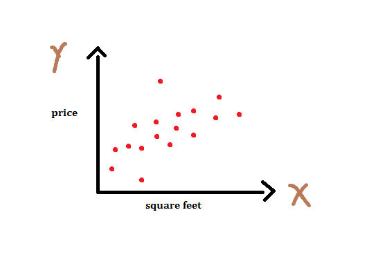
Apparently, we can fit n number of lines by tweaking coefficients m and b as shown below. line fitting

We can rewrite our equation as y(x) = w₀ + w₁ * x where, w₀ is the bias term and w₁ is the slope. Here, w_i’s are known as the weights or parameters of our model. This equation can be used when we have one input variable (feature or independent variable) and this is called as simple linear regression . But this is not the ideal case. We usually deal with the datasets which have many features, the case when we have more than one features it is known as multiple linear regression . We can generalize our previous equation for simple linear regression to multiple linear regression - $y(x) = w_0 x_0 + w_1 x_1 + w_2 x_2 + ... + w_n x_n$ . Here, x₀ = 1 ( intercept term ) and w₀ , as I mentioned earlier, is the y axis intercept. To simplify the notation, we rewrite the above equation as follows: $y(x)\) = \(\sum\limits_{i=0}^n w_i x_i = w^Tx$

By changing the weights we can get different lines and now our task is to find weights for which we get best fit. One question you might have is, how can we determine how bad or good a particular line fits our data?. For this, we introduce a cost function which measures, for each value of w’s, how close the y’s are to corresponding y_true’s. We define our cost function as simple sum of sqaured error. Here, 1/2 is added to make derivation easy as we will see later.

$J(w)\) = \(\frac{1}{2}\sum\limits_{i=1}^n (y(x^i) - y_t^i)^2$

As I mentioned earlier, this cost function calculates how far y’s are from the corresponding y_true’s. We can show this in the graph as shown in figure - 3. Basically, our cost function calculates the distance between true target and predicted target which is shown in the graph as lines between sample points and the regression line. This is called residual.

cost function visualization

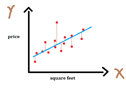
For each value of weight, there will be some cost or an error. We want to find the value of weights for which cost is minimum. We can visualize this as follows :

gradient descent

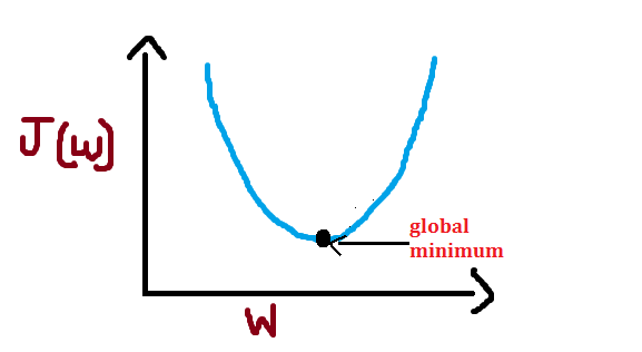
As you can see, we get some value of cost/error for each value of weight. Here, I have used the word “global” and the reason is- In case of non-convex shape there will be more than one minimum but we want to find out the global minimum. For simplicity, I have used convex shape in above figure.

Gradient Descent

Essentially, what we do in supervised learning problems is finding the best weights for our model. Hence, our task becomes an optimization task. Gradient Descent is one of the most popular and widely used optimization algorithm. Gradient descent can be used to minimize a cost function $J(w)$ parameterized by a model’s parameters $w \in \mathbb{R}^d$ by updating the parameters/weights in the opposite direction of the gradient of the cost function $\nabla_w J(w)$ w.r.t to the parameters. Mathematically we can write as
$w_n = w - \eta \cdot \nabla_w J( w)$

Here, $\eta$ is the learning rate which determines the size of the steps we take to reach a minimum. We need to be very careful about this parameter since high value of $\eta$ may overshoot the minimum and very low value will reach minimum very slowly.

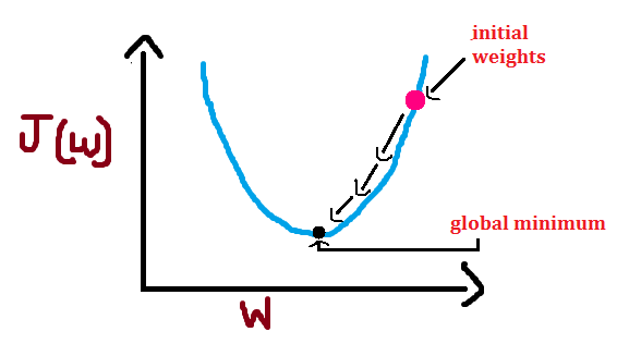
There are three variants of gradient descent- Batch Gradient Descent, Stochastic Gradient Descent and Mini-batch Gradient Descent. Batch gradient descent computes the gradient of the cost function w.r.t to parameter w for entire training data. Since we need to calculate the gradients for the whole dataset to perform one parameter update, batch gradient descent can be very slow. Stochastic gradient descent computes the gradient for each training example $x^i$ . Mini-batch gradient descent computes the gradient for every mini-batch of m training example. If you are curious about gradient descent and its variants then check out this post by Sebastin Ruder.

In order to complete this algorithm we have to calculate the partial derivative term $\nabla_wJ(w)$ . Let us first derive equations for one training example and later we will modify it for more than one training example.

$\nabla_wJ(w)\) = $\frac{\partial}{\partial w_j} J(w)$ = \(\frac{\partial}{\partial w_j} \frac{1}{2} ( y(x) - y_t))^2$

$= \(2 \cdot\frac{1}{2} (y(x) -y_t) \cdot\frac{\partial}{\partial w_j} (y(x) - y_t)$

$= $(y(x) - y_t) \cdot\frac{\partial}{\partial w_j} (\sum\limits_{i=0}^n w_i x_i - y_t)$$

$= $(y(x) - y_t) x_j$$

Now, we can rewrite our update rule as follows :
$$w_n$ = $w - \eta \cdot (y(x) - y_t) x_j$ (Repeat until convergence)$

We can modify this equation for more than one training example as follows :
$w_n\) = \(w - \eta \cdot \sum\limits_{i=1}^n (y(x) - y_t) x_j$

Note that we are updating our weights after going through entire dataset, that is, at each step we iterate through entire training dataset and then we update the weights. Can you recall the name of this variant of gradient descent? This is, Batch Gradient Descent. Please note that some people use term vanilla gradient descent instead of batch gradient descent. For stochastic gradient descent, we just need to remove the summation symbol from above equation. In practice, we use mini-batch gradient descent which takes best of both and performs update after going through a batch of n example. For mini-batch gradient descent, we can write update rule as:

$w_n = w - \eta \cdot \nabla_w J( w ; x^{(i:i+n)} ; y^{(i:i+n)})$

There are some challanges with aforementioned gradient descent algorithms such as choosing a proper learning rate. Researchers have proposed several methods to solve this problems such as adam, adagrad, RMSProp. Please read this excellent blog post to understand those challenges and gradient descent optimization algorithms.

Summary

Seems like too much work for this simple linear regression, but believe me it’s not, it’s very easy. Let me briefly write some takeaways,

For simple linear regression, equation of line is y(x) = w₀ + w₁ * x₁. Here, w₀ is the intercept term and w₁ is the slope of the line. We want to find w₀ and w₁ such that it minimize our cost function. We can easily extend this equation for multiple linear regression as shown above.
We start with small positive random weights .
Calculate the loss/cost/objective function as follows :
$J(w)\) = \(\frac{1}{2}\sum\limits_{i=1}^n (y(x^i) - y_t^i)^2$
We update our weights as follows :
$w_n\) = \(w - \eta \cdot \sum\limits_{i=1}^n (y(x) - y_t) x_j$ (we derived this equation above)
Repeat steps 3 and 4 until convergence. In other words, repeat step 3 and 4 until $J(w)$ < 0.0003. The number 0.0003 was chosen randomly. Please note, we do not need cost function to calculate weight update since we have derived a equation (step -4) which does not depend on cost function. But its always a good idea to print cost so that we can keep track of how well our model is doing (i.e cost is decreasing or not). If we change the cost function, we have to modify this weight update rule.

Logistic Regression

Logistic Regression is the special case of linear regression where dependent or output variable is categorical. Don’t be confused by the name of logistic regression, its a classification algorithm. Logistic in logistic regression comes from the function which is the core of this algorithm. This function is logistic function or sigmoid function . Logistic function can be written as :

$y(z)\) = \(\frac{1}{1 + e^{-z}}$

We can plot y(z) as follows :

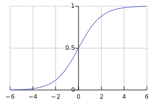
A sigmoid function squashes the input value between [0,1] so that we can interpret output as a probability. One desirable property of sigmoig function is that it is differential and it has non-negative derivative at each point.

In linear regression we used linear equation ( $w_0 + w_1 x_1$ ) as our hypothesis. But certainly its not a good choice when output is categorical variable such as binary-values variable ( $y^i \in \{0,1\}$ ). In logistic regression, we use different hypothesis class which predicts the probability of an each class. Class with highest probability is the predicted target. For example, if we want to build a classifier that classifies an email as spam or ham then logistic regression model assigns a probability to both class (spam and ham) say 0.7 to spam and 0.3 to ham then our output will be spam. Mathematically we can write out hypothesis function as follows :

$\begin{align}P(y=1|x) & = h_w(x) = \frac{1}{1 + \exp(-w^\top x)} \equiv \sigma(w^\top x),\\P(y=0|x) &= 1 - P(y=1|x) = 1 - h_w(x)\end{align}$

where $\sigma$ is the sigmoid function.

Now, our task is to find the weights for which P(y=1|x) is large when input belongs to the class 1 and small when input belongs to the class 0. We need a cost function to measure how well a model performs, here we use negative log-likelihood :

$\begin{align} J(w) = - \sum_i \left(y^{(i)} \log( h_w(x^{(i)}) ) + (1 - y^{(i)}) \log( 1 - h_w(x^{(i)}) ) \right)\end{align}$

Here, we will use gradient descent to optimize a model. Our task is to learn a weight for which cost is minimum. After training, we can predict the class by calculating probability of each class. Class with the highest probability will be assigned as a target/output. For binary-valued labels, if $h_w(x) > 0.5$ then the class is 1 otherwise 0.

Derivation of a cost function is the same as it was in linear regression (check it out). The only difference is that hypothesis function is changes with sigmoid function.
$\nabla_w J(w)\) = \(\sum_i x^{(i)} (h_w(x^{(i)}) - y^{(i)})$

Where, y is a true class.

Overfitting

One of the most important problem in the machine learning is called Overfitting. Overfitting happens when a model performs too well on training data but does not perform well on unseen data. It happens when a model learns the noise present in the training data. Conversely, when a model does not perform well on training data as well as unseen data then that is known as Underfitting. If our dataset is very small then there will be a high chance of overfitting. The reason is, when the size of training example is small our model will simply memorize it instead of learning from it. In the following part, we will see ensemble methods which are good learners in case of small dataset. In ensemble methods, instead of training one model we train multiple models and average the predictions.

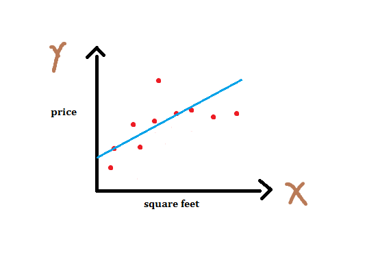
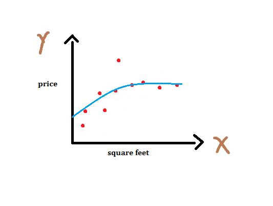
If we fit $y\) = $w_0 + w_1 x_1$ to a dataset, we get the straight line as shown above in figure - 6. Note that this is not a good fit since it does not pass through many points. This is the instance of underfitting. Now, if we add another feature x² and fit $y$ = \(w_0 + w_1 x_1 + w_2 x^2$ then we’ll get fitting as shown below in figure -7. This is slightly better than previous since it passes through several points.

If we add more features we’ll get better fit. Below figure shows an instance of this case. This is overfitting. Note that it’s polynomial fitting and we can represent n-th order polynomial as $y\) = \(\sum\limits_{i=0}^n w_i x^i$ .

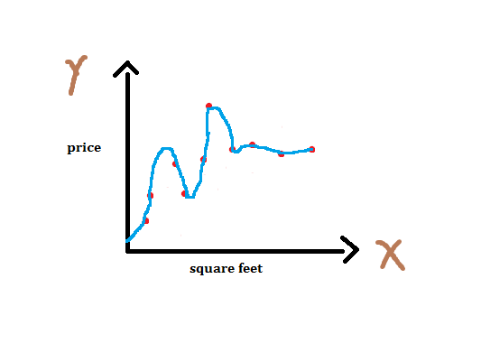
Even though fitted curve passes through almost all points, it won’t perform well on unseen data. It has just memorized the training data. Several ways to avoid overfitting are : 1 - Use more data 2 - Apply cross-validation 3 - Regularization

Regularization

Next, we will see various regularization techniques. Regularization refers to the method of preventing overfitting, by controlling the model’s complexity. The concept behind regularization is to introduce additional information to penalize extreme weights.

L2 regularization is the commonly used regularization technique. In linear regression overfitting is characterized by large weights. By adding penalty term in our objective function we can control the complexity or the magnitude of the weights. In L2 regularization we penalize squared magnitude of all weights. We can rewrite our cost/objective with L2 regularization as follows :
$J(w)\) = \(\frac{1}{2}\sum\limits_{i=1}^n (y(x^i) - y_t^i)^2 + \frac{\lambda}{2} ||w^2||$ where $\lambda$ is the regularization strength.

L1 regularization is the same as L2 with the only difference that instead of adding $\frac{\lambda}{2} ||w^2||$ to each weight w we add $\frac{\lambda}{2}||w||$ .
$J(w)\) = \(\frac{1}{2}\sum\limits_{i=1}^n (y(x^i) - y_t^i)^2 + \frac{\lambda}{2} ||w||$

One interesting property of L1 regularization is that model’s parameters become sparse during optimization. If you don’t want this property in your model then L2 regularization is always preferred over L1 regularization. Please note, ordinary least square (which we saw earlier in linear regression) with l2 regularization is known as Ridge Regression and with l1 regularization it is known as Lasso Regression.

Cross Validation

One of the critical task in machine learning is model evaluation, that is, to test how well a model performs on unseen data. Here, we will see Cross Validation which is the model evaluation method. It’s not a good idea to test our model on a dataset which we used to train a model since it won’t give any indication of how well our model performs on unseen data, in other words, how well our model generalizes to unseen data. Generalization is the desirable characteristic we want in a model. We can overcome this problem by not using entire training data while training a model. Instead we will hold out some data (test data) and we’ll train only on remaining data. Once the training is over we can use test data to test the performance of a model. For example, we can split our whole dataset into 70/30 ratio. That is, we use 70% data to traing and 30% data to test a model.

The holdout method is the simplest kind of cross validation method. Which exactly what I explained above. We split our dataset into two parts, training and testing datasets. We use training dataset to train a model and testing dataset to evaluate the performance of a model.

In K-fold cross validation , the dataset is divided into k seperate parts. We repeat training process k times, each time, holding out one subset to test a model and remaining data can be used to train a model. Then we average the error to evaluate a model.

The Leave-one-out cross validation is the special instance of k-fold cross validation. In which, k is equal to the number of data points in the dataset. Each time, we hold out a single data point and train a model on rest of the data. We use this one data point to test our model. Then we calculate the average error to evaluate a model.

Learning = Representation + Evaluation + Optimization

You might have concluded in your mind that supervised learning is all about finding weights which minimize our cost. And that’s true. But let us dig deeper and gain some insights on how learning really works. We will discuss this in depth for the classification problems since they are the widely used ones. We can divide learning phase in three parts - Representation, Evaluation and Optimization.

Representation : Choosing a representation of a learner is tantamount to choosing the set of classifiers that it can possibly learn. This set is called hypothesis space.
Evaluation : An evaluation or objective function is needed to distinguish good classifiers from bad ones.
Optimization : We need a method to find the best classifier in hypothesis space. Here comes the optimization. The choice of optimization technique determines the efficiency of a learner. Gradient descent optimization technique which we discussed earlier is the first-order optimization technique.

In this part, I explained what machine learning is, different types of machine learning, linear regression and several methods to make it more accurate. You can find code for this part here. In the next part, I will explain Naive Bayes, Support Vector Machine and tree based algorithms. If you have any query or feedback kindly write me at vsavan7@gmail.com. You can follow me on twitter to get updates on new parts of this series.